Learning Where to Simulate
Generative Active Sampling for Online PDE Surrogate Training
From solvers to online active learning
A PDE solver
A classical PDE solver is a function F that produces the state at the next time step from the current one and some parameters λ:
Xt+Δt = F(Xt, λ)
Starting from an initial condition X0, it produces a trajectory X0, …, XT. A neural surrogate Fθ learns to imitate F, orders of magnitude faster.
Classical surrogate training
The usual practice first builds a dataset: initial conditions and parameters (X0, λ) are sampled uniformly, and the solver generates the corresponding trajectories. Fθ is then trained on this fixed dataset over many epochs. But a uniform draw likely leaves the hard-to-learn trajectories under-represented. Think of a fluid solver parametrized by its viscosity: high-viscosity regimes are smooth and easy to learn, low-viscosity ones can become turbulent.
Online active learning
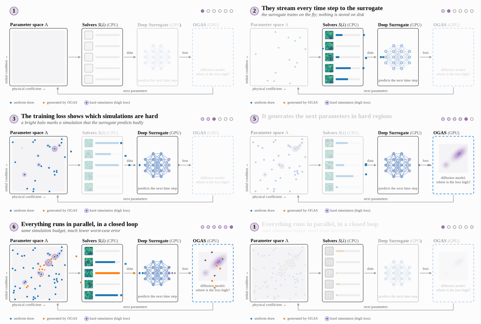
The first step is online training. Instead of learning from a fixed dataset, the solvers run concurrently with the training: each new state is streamed to a buffer from which the training draws its batches, and a solver that finishes a trajectory picks a new (X0, λ) for the next one.
Data production can then follow the progress of the training. A training signal, such as the surrogate loss, shows where the training struggles, and this information is used to generate the next (X0, λ) towards hard-to-learn trajectories. This kind of active learning, where samples are generated rather than selected from a pool of candidates, is called query-synthesis. The difficult question is how to design the sampling policy: this is what OGAS is about.
Where the difficulty comes from
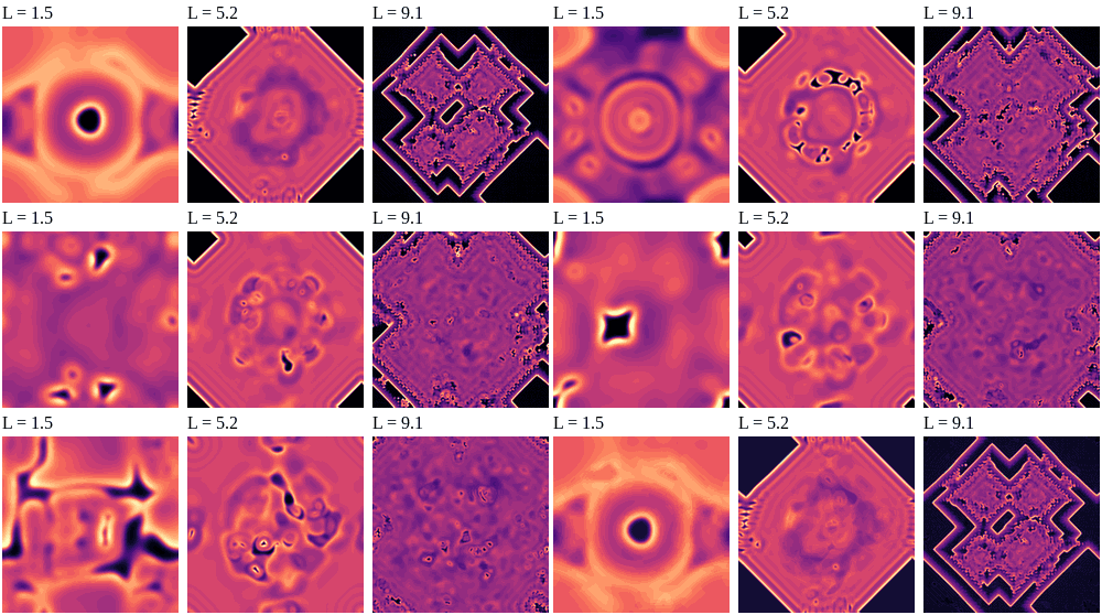
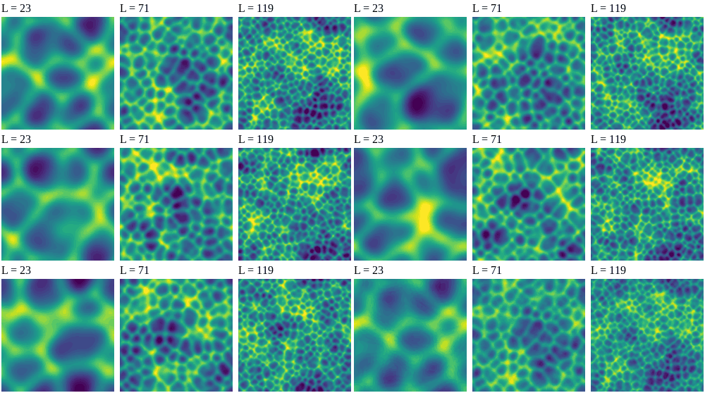
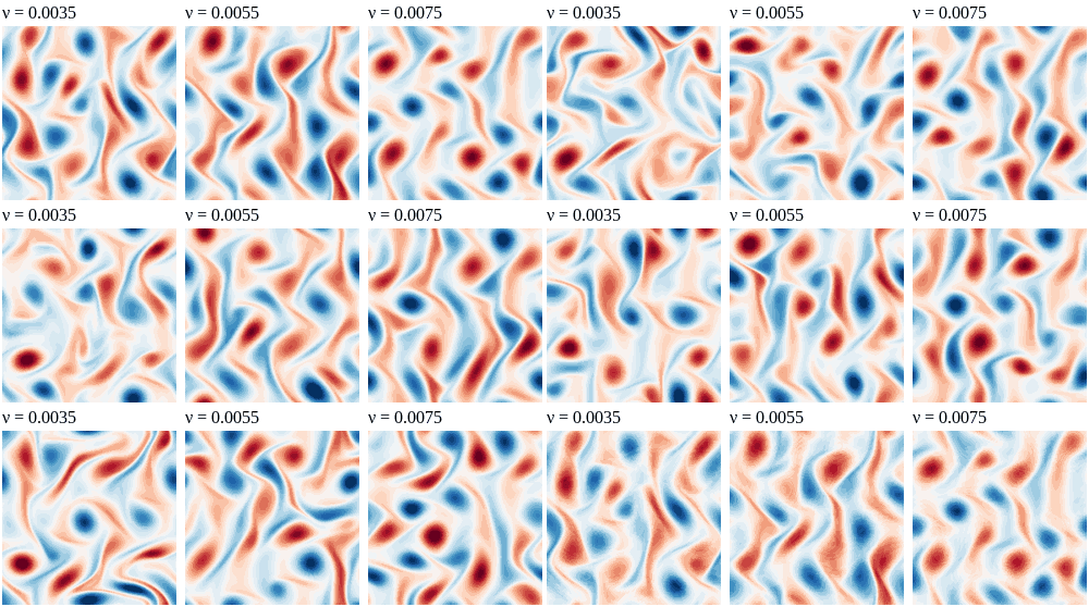
Our three benchmarks make this concrete. A simulation is defined by a physical coefficient and a parametrized initial condition, and the coefficient alone changes the dynamics qualitatively. Each row shows one PDE at a low, a middle and a high value of its coefficient.
Gray-Scott
Reaction–diffusion of two chemicals. The domain size L ∈ [0.5, 10] goes from a few large spots to fine, ever-changing patterns.
Initial condition: 8 Gaussian blobs (48 parameters).
Kuramoto–Sivashinsky
Chaotic dynamics. A larger domain size L ∈ [10, 130] packs more and smaller cells into the same 256×256 grid.
Initial condition: truncated Fourier series (308 parameters).
Kolmogorov flow
Forced 2D turbulence (Navier–Stokes). The viscosity ν ∈ [0.003, 0.008] (Reynolds 125–330) changes the dynamics more subtly.
Initial condition: truncated Fourier series (308 parameters).
What OGAS samples
OGAS answers this question with a generative model that learns where the training struggles. Each finished simulation receives a difficulty score: the training loss it produced (OGAS-Loss) or the disagreement of two surrogates on it (OGAS-Uncertainty). A small diffusion model (a conditional DDPM) learns from the recent pairs of parameters and scores, and OGAS asks it for parameters with a high target difficulty: these become the next simulations. It runs alongside the training, on its own GPU.
Training starts with 100 % uniformly sampled parameters; as it progresses, generated ones are mixed in, up to 70 %. The remaining 30 % of uniform samples keep exploring the space, to find the next hard regions as the current ones get learned and to avoid forgetting the easy ones, while the generator exploits what the training has revealed.
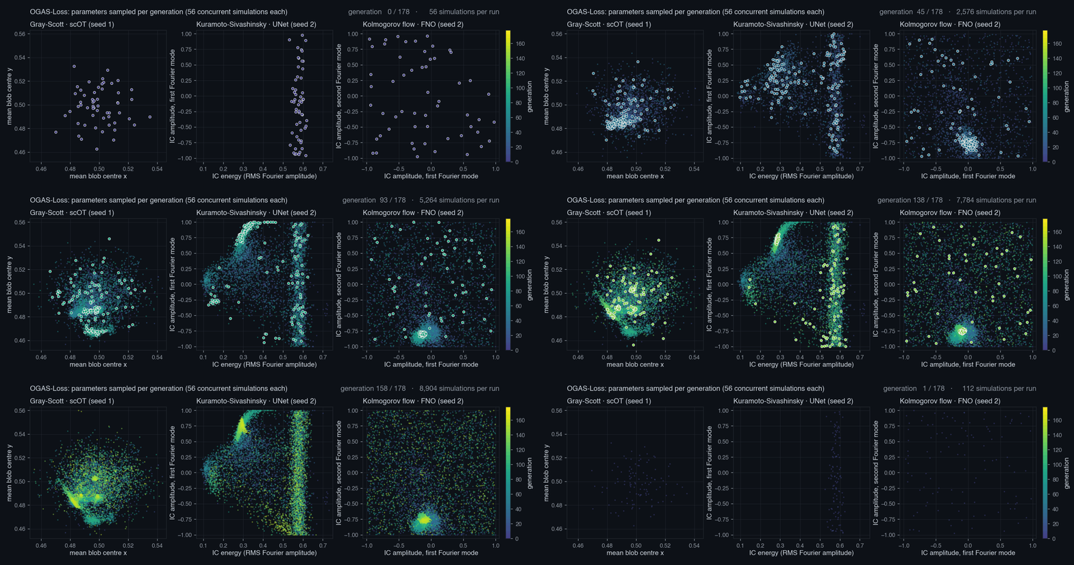
The plots below show how the requested parameters evolve during one training run. Starting from well-spread, uniform samples, they progressively concentrate on specific regions, the hard-to-learn ones.
Results
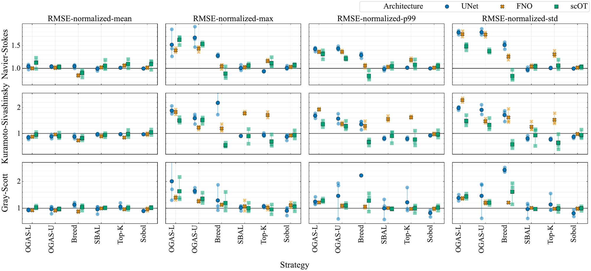
OGAS is compared with uniform and Sobol sampling, pool-based active learning (SBAL, Top-K) and an online Gaussian-mixture sampler (Breed), all at the same simulation budget and the same number of gradient steps.
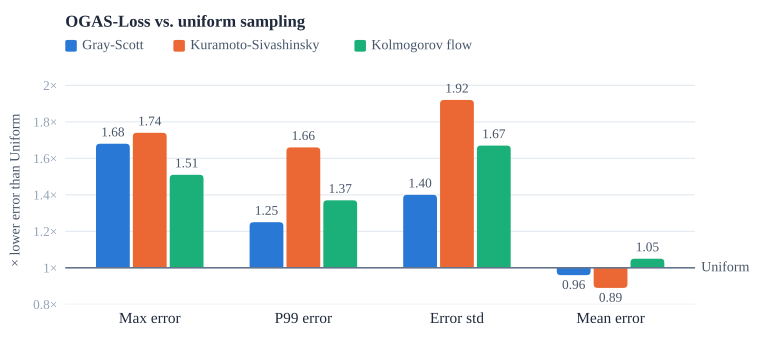
The gain is concentrated in the tail: the worst errors and their spread shrink, at a small cost on the mean error, which a uniformly drawn validation set weighs towards easy regimes. SBAL, Top-K and Sobol give smaller or inconsistent gains.
On a second validation set drawn from the OGAS generator itself (750 trajectories per PDE, UNet), OGAS-Loss improves every statistic, the mean included: the mean error drops by 1.08× to 1.38× and the 99th percentile by 1.22× to 2.16×. Both surrogates make larger errors on this set: the configurations OGAS finds hard are also hard for a uniformly trained surrogate.
Where the gain comes from
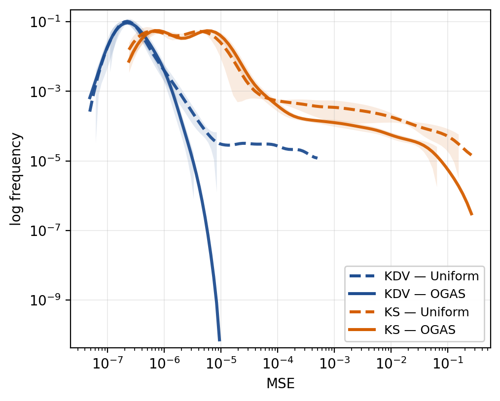
The full error distributions show where the gain comes from: OGAS and Uniform match on most validation samples, but OGAS makes far fewer large errors, with the density of the high-error tail dropping by orders of magnitude reducing the risk of a high step error.
Debiasing the sampler
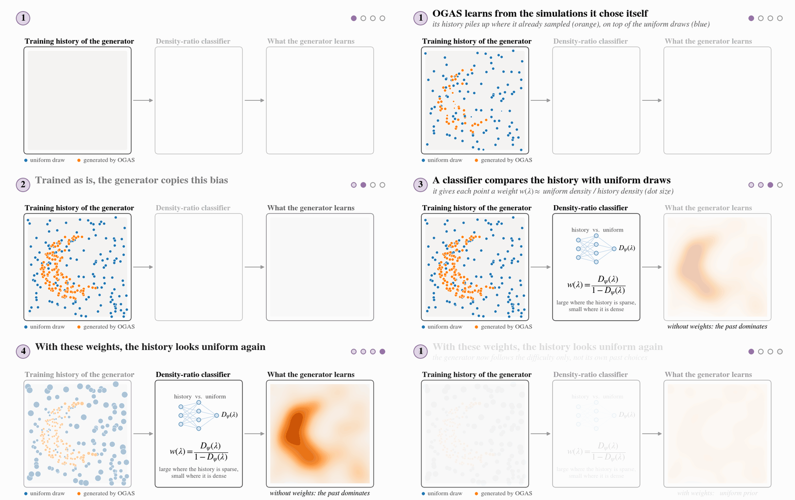
Because of the online closed loop, the DDPM ends up learning from simulations it chose itself, so its training history over-represents the regions it already favored. A classifier estimates how much denser the history is than a uniform draw. The DDPM's training examples are weighted by the inverse ratio, which mitigates this closed-loop sampling bias: the DDPM (not the surrogate) trains on a corrected distribution leaning toward a uniform prior.
Implementation
OGAS is built on Melissa, a framework for training neural networks online from simulations running on HPC clusters. Melissa launches the solvers, streams their states to the training through an in-memory buffer instead of the disk, and keeps simulation and training running concurrently; OGAS plugs its sampler into this loop, on its own GPU.
The code of the experiments, with the configurations and scripts to reproduce the paper, is on GitHub.
BibTeX
@inproceedings{cesar2026learning,
  title     = {Learning Where to Simulate: Generative Active Sampling for Online {PDE} Surrogate Training},
  author    = {Cesar, Pierre and Dymchenko, Sofya and Purandare, Abhishek and Raffin, Bruno},
  booktitle = {Advances in Neural Information Processing Systems (NeurIPS)},
  keywords  = {active learning, online training, surrogate modeling, partial differential equations, generative models},
  pages     = {1--10},
  month     = dec,
  year      = {2026},
  address   = {Paris, France}
}